Calculating Slope on a Tiled Dataset, Part 1

The Problem

PostGIS supplies us with a nice function, ST_Slope, that quickly calculated slope from a DEM. However, we can’t calculate slope at the edge of a raster, because we need neighboring pixels on all sides of our targeted pixel to calculate its slope. With tiled rasters, I think we can expect to encounter this problem frequently.

This post is all about testing how PostGIS responds to that problem.

Hypothesis

This post is just an initial examination of what happens when we calculate slope on a tiled DEM.

My hypothesis: we’ll see edge effects at every tile boundary unless we use ST_Union.

If this is the case, then we have to turn our minds to solving the problem. One way that jumps to mind initially would be to tile the DEM at a resolution that would work for the output

Let’s see what really happens!

Getting Started

The Data

I’ll be using ASTER GDEM v2* for this test. If you’d like to follow along you will need an actual DEM since we’re calculating slope, rather than the simulation approach I’ve encouraged in some of my other posts. You can use the same data I’m using by downloading it from LDAAC GDEx or NASA Reverb after creating a free account. J-spacesystems used to distribute it as well, though they ceased doing so in 2016. I highly recommend Reverb, and there’s a good guide on how to download it here.

If you’re not familiar with ASTER GDEM, it’s supposed to be the higher-resolution successor to SRTM. However, there are many issues with the data. I’ve written about some of them if you’d like to learn more.

Pick an Area

I’ve got GDEM v2 for most of the globe, so I’m going to select a subset of the data. It doesn’t really matter where, but I want something with some interesting topography. I tiled GDEM at 100x100 when I pulled it in, so we won’t need to do that.

1
2
3
4
5
6
7
8
9
10
11
12
13
14
15
16
17
18
19
20
21
22
23
24
25
26
27
28
29

-- New table for new data
CREATE TABLE public.dem_foco_100 (
  rid SERIAL primary key, rast raster
);
-- Select an area within 30km of downtown Fort Collins
INSERT INTO dem_foco_100(rast)
SELECT rast
FROM gdem_100
WHERE ST_Intersects(
  ST_Envelope(rast)  -- Raster tile bounding box
, ST_Envelope(       -- Get a bouding box
    ST_Buffer(       -- Of a buffer
      ST_SetSRID(    -- Of a point in downtown FOCO
        ST_MakePoint(-105.085670, 40.572171)
        , 4326)::geography  -- Note the use of the geography type
      , 30000)::geometry)   -- The buffer radius is 10,000m. We
                            -- convert back to geom to get BB.
);
-- Constrain and index rasters to improve query speed
SELECT AddRasterConstraints(
  'foco_dem_100'::name,  -- table
  'rast'::name  -- raster geometry column
);
CREATE INDEX foco_dem_100_gist_idx
ON foco_dem_100
USING GIST(ST_ConvexHull(rast));

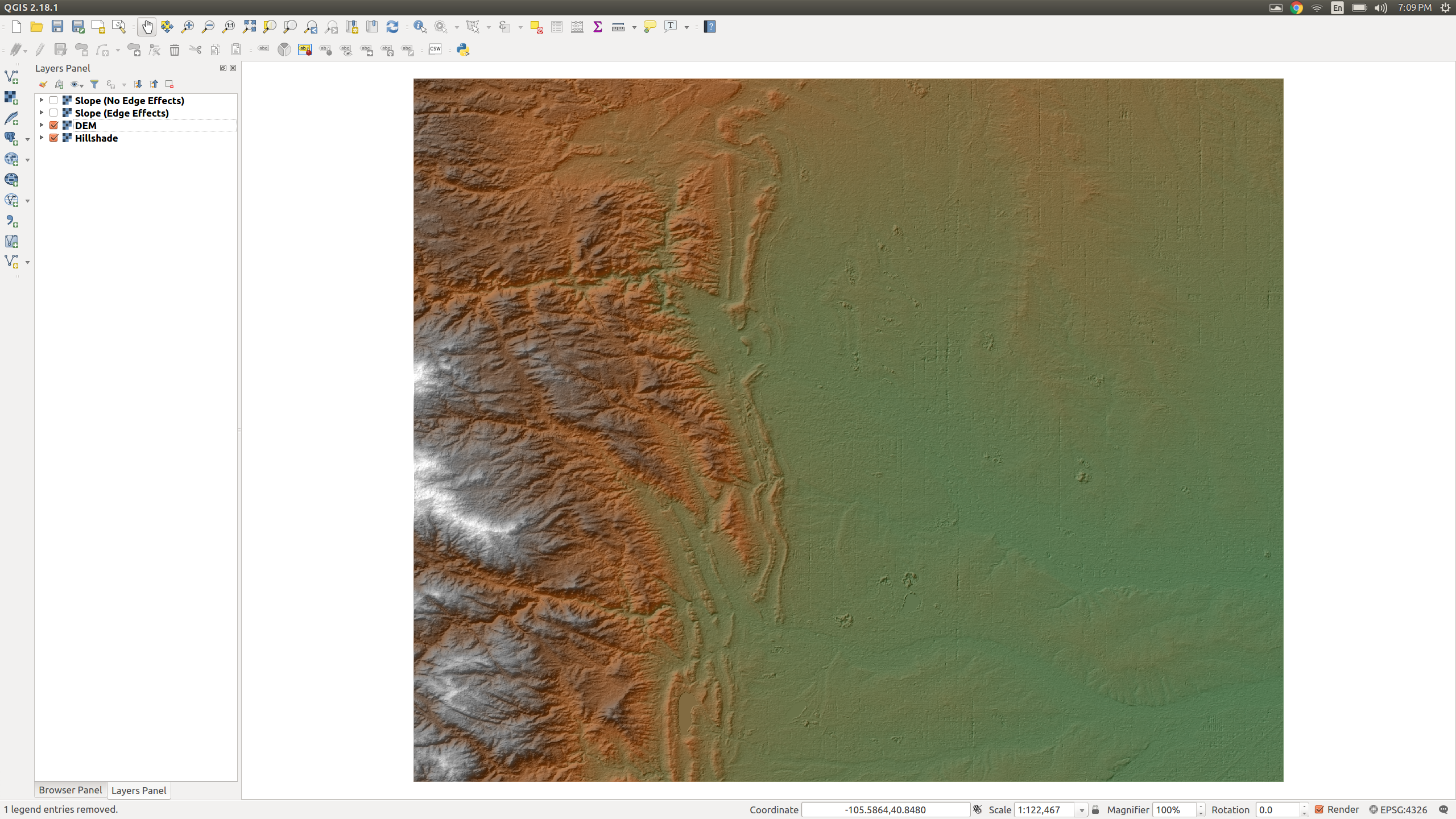
This query selects a the area around Fort Collins, Colorado, USA. Specifically, I’ve selected all raster tiles that intersect the bounding box of a 30km buffer around Colorado State University.

View full size

Notice that I used the geography type in the query above. I did this so I could specify my buffer length in meters, rather than degrees. Using the geography variant of ST_Buffer (the final variant listed here) of the function, as the docs explain, can cause some problem with geometries that cover large areas, but I think it’s worth the convenience in this case.

Hit the Slopes

First Attempt

Alright, with our subset selected, let’s try out the operation and see what we get. Here, we’ll get the slope for a 10km area around CSU.

1
2
3
4
5
6
7
8
9
10
11
12
13
14
15
16
17
18
19
20

CREATE TABLE public.slope_foco_100 (
  rid SERIAL primary key, rast raster
);
INSERT INTO slope_foco_100(rast)
SELECT ST_Slope(
  rast,
  1,              -- Band
  '32BF',         -- Pixel Type
  'DEGRESS',      -- Slope units
  111120,         -- Scale (convert Lon/Lat to Meters)
  FALSE::boolean  -- Interpolate nodata?
)
FROM dem_foco_100
WHERE ST_Intersects(
  ST_Envelope(rast)
, ST_Envelope(
    ST_Buffer(ST_SetSRID(ST_MakePoint(-105.085670, 40.572171), 4326)::geography
      , 10000)::geometry)
);

Okay, time to pop over to QGIS and see what we’ve got!

View full size

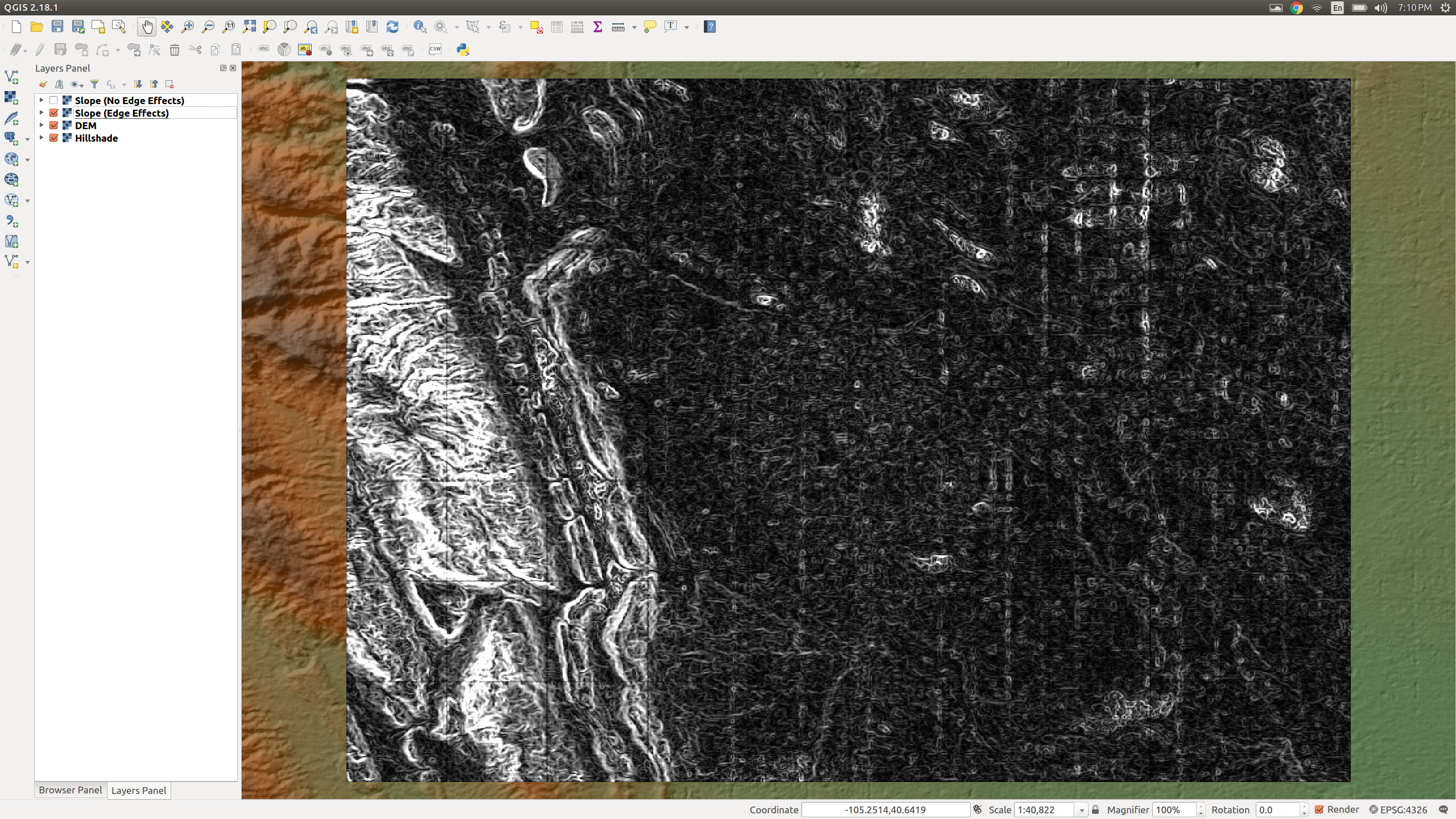
Well, shoot. See the weird grid that shows up in the slope area? Looks like we have edge effects.

I’d expected that, but you can always hope you’re wrong about these kind of things! Let’s figure out what we can do about it.

Second Attempt

Since we’re having trouble with the edge effects, one thing we can do is get rid of the edges.

Using ST_Union, we can combine all the tiles into a single raster befoe we calculate slope on it. This way, we will only have problems at the very edge of our study area where they’re not as impactful.

1
2
3
4
5
6
7
8
9
10
11
12
13

CREATE TABLE public.slope_good_100 (
  rid SERIAL primary key, rast raster
);
INSERT INTO slope_good_100(rast)
SELECT ST_Slope(ST_Union(rast), 1, '32BF', 'DEGRESS', 111120, FALSE)
FROM dem_foco_100
WHERE ST_Intersects(
  ST_Envelope(rast)
, ST_Envelope(
    ST_Buffer(ST_SetSRID(ST_MakePoint(-105.085670, 40.572171), 4326)::geography
      , 10000)::geometry)
);

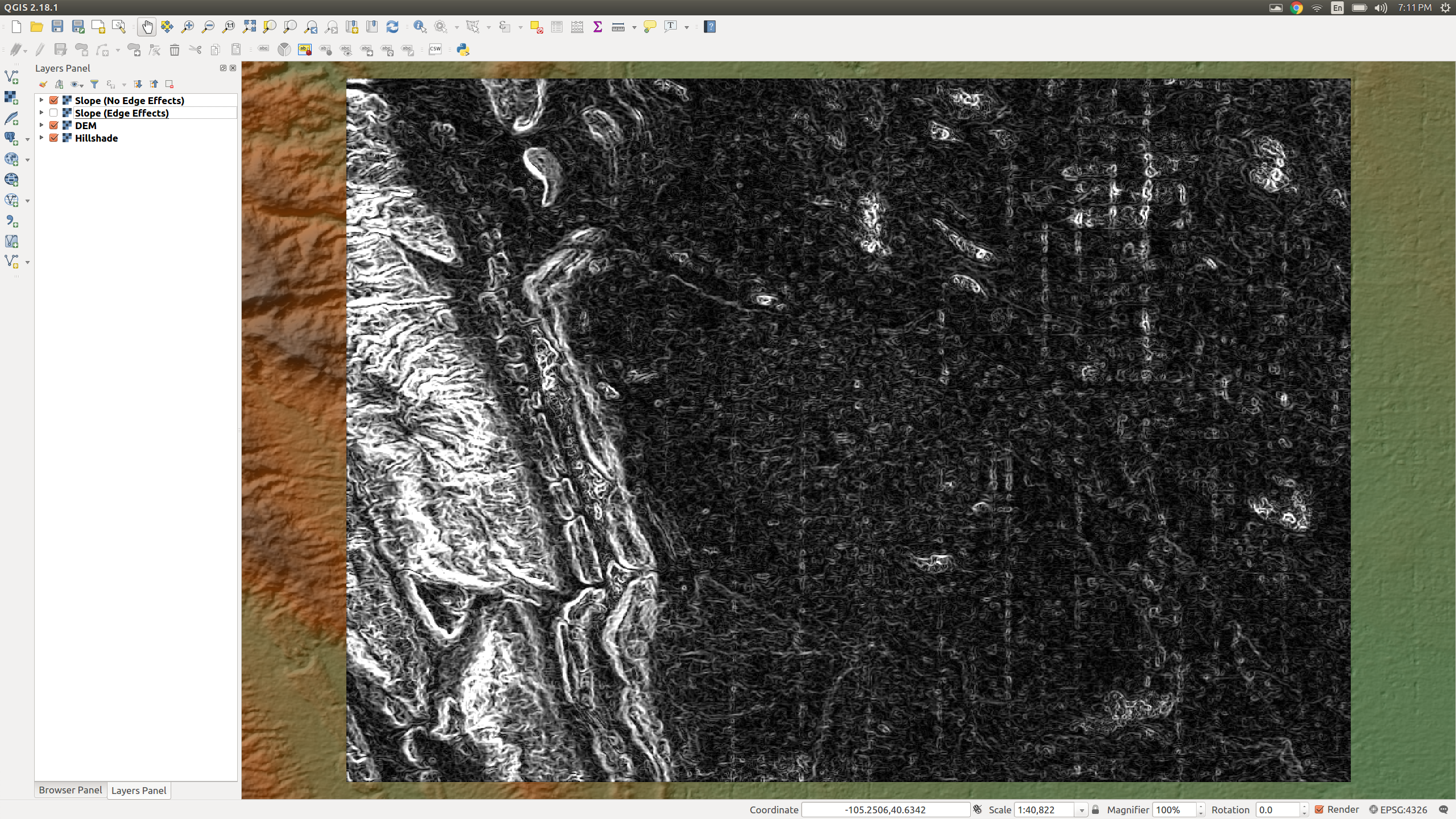
Back in QGIS, we can see that the this time around, we don’t have the weird grid! Hooray!

View full size

Conclusions

We can easily avoid the problems created when calculating slope on a tiled DEM with the powers of ST_Union. Great news! Proceed with your analysis. In fact, download the code from this post as a guide to help you!

But what if you need to get the slope for an extremely large area, like, say, the whole world? You can’t just SELECT ST_Union(rast) the entire globe, it’s too much data! We’d need a way to work through it bit by bit, calculating slope one tile at a time.

I face that exact problem in my thesis research. I’m working on a blog post about it now. Stay tuned for more! I’ll update this post with a link when I finish it.

*ASTER GDEM is a product of METI and NASA.